BlazeSeg

Implementing and training a simple sub-millisecond semantic segmentation model.

Figure 1 BlazeSeg results for person foreground segmentation. The model can run inference on \(128\times 128\) images in less than \(1\text{ms} ^{\dagger}\). Video source\(^{\ddagger}\).

I recently read and implemented the paper "BlazeFace: Sub-millisecond Neural Face Detection on Mobile GPUs". The paper shows how one can perform sub-millisecond face detection on mobile devices. I checked if there was a semantic segmentation version using the same "Blaze" philosophy, but I did not find an explicit one (only the MediaPipe paper and website).

Having already written a pytorch version of the Blaze backbone, I decided to extend it to perform semantic segmentation and see how well it performed. I called the model BlazeSeg.

Model Architecture

The Blaze decoder is based on a simple CNN architecture that processes a \((3 \times 128 \times 128)\) image. The key idea is the use of group convolutions to learn features over the spatial dimension and point-wise convolutions along the channel dimension. Compared to a standard convolution, this is very efficient as it has fewer total parameters and operations.

The Blaze decoder downsamples the image by a factor of \(16\). As we are performing semantic segmentation, we need to upsample the image to the original size as shown in Figure 2.

Figure 2 Overview of the BlazeSeg architecture. A full model description is available here.

In this setting, the choice of upsampling boils down to essentially a transposed convolution or a form of interpolation. Since the goal is to have a very fast model, I decided to first benchmark which of the two operations was faster (Table 1). To my surprise, bilinear upsampling is significantly faster than transposed convolution, so I opted for it.

Operation	CPU (avg)	CUDA (avg)	Calls
`conv_transpose2d`	61.219μs	47.755μs	4000
`upsample_bilinear2d`	17.796μs	20.012μs	4000

Table 1 Latency comparison between transposed convolution and bilinear upsampling on CPU and CUDA\(^{\dagger}\).

An upsampling block first bilinearly upsamples the input feature map and then projects the input channels into the target output dimension. Afterwards, the possible skip connection is concatenated along the channel dimension and a group and point convolution are applied. The model in total has \(0.160681\text{M}\) parameters.

Model Training

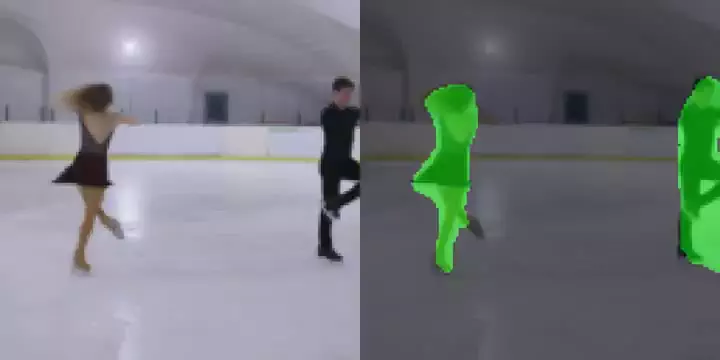
I decided to train the model to perform person segmentation. After a brief look online for datasets I decided to use this Kaggle dataset as it has about \(5\text{k}\) images with segmentation masks.

I trained the model using the Binary Cross Entropy loss. As the number of background pixels usually outnumbers the foreground ones, I also used a simple positive weighting factor: \(w_\text{pos} = \frac{\text{# background}}{\text{# foreground}}\).

I trained for \(100\) epochs with a constant learning rate of \(0.001\) and a batch size of \(8\). I obtained similar results when using a cosine annealing scheduler. Admittedly, this was not a very extensive parameter search, and better performance could probably be reached with more effort.

As checkpoint selection metrics I used both the train and validation losses and the Binary IoU on the validation set (Figure 3 shows an overview). The selected checkpoint reached \(\approx0.7124~\text{mIoU}\).

Figure 3 Metrics derived from training and validation.

Model Analysis and Deployment

Let's first see how this architecture scales with the number of output classes. As this only affects the last convolutional layer, the impact on the model inference time and size is relatively small (shown in Figure 4).

Figure 4 Impact of the number of output classes on the model inference runtime and GPU model size\(^{\dagger}\).

As can be seen in Figure 4, the model inference time, even with a single output class, is well above the \(1\text{ms}\) threshold. To get below the threshold, I decided to export the model using torch-TensorRT in order to efficiently run the model on my NVIDIA GPU.

Backend	Runtime (mean)	Runtime (std)	CUDA Memory (mean)
`PyTorch (CPU)`	10.2325 ms	0.8751 ms	–
`PyTorch (CUDA)`	1.8946 ms	0.0919 ms	0.82 MB
`TensorRT FP32`	0.6627 ms	0.0822 ms	0.19 MB
`TensorRT FP16`	0.6291 ms	0.0828 ms	0.19 MB

Table 2 Runtime and CUDA memory comparison between pure PyTorch and TensorRT inference backends. The PyTorch models use FP32. The TensorRT models run on CUDA\(^{\dagger}\).

As shown in Table 2, TensorRT reduces runtime by \(\approx66.7\%\) and model size by \(\approx76.8\%\). Given how easy it is to export a model the switch to TensorRT seems like a good deal.

Misc

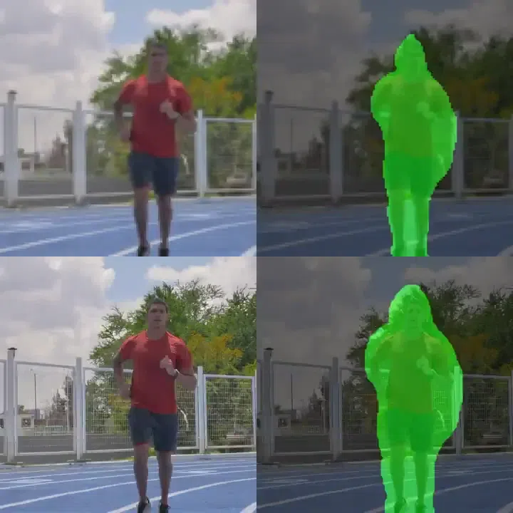
While \(128\times128\) images are not particularly high resolution, running the model on higher-resolution inputs would inevitably increase the runtime. A possible compromise could be running the model inference on the small resolution and then upsample the output mask to the desired one (see example in Figure 5).

Figure 5 Qualitative results of running the model on low-resolution images (top) and upscaling the output mask with additional smoothing (bottom).

\(\dagger\) All GPU measurements were performed using an NVIDIA GTX 1650 4GB mobile. All CPU measurements were instead performed on an AMD Ryzen 7 4800H.

\(\ddagger\) Video source is this.